
From Data to Discovery: A Step-by-Step Walkthrough of the Harmonic TDA Pipeline
The Inverse problem of TDA, Solved.


1. Introduction: The “Right to Left” Challenge in TDA
In the standard Topological Data Analysis (TDA) pipeline, the workflow is linear: we move from raw data to a geometric structure, and finally to a barcode, a persistence diagram summarizing the “holes” across scales. However, a significant bottleneck arises when we attempt to move “right to left.” If a specific bar in a barcode represents a critical structural pattern, how do we identify the specific data points (e.g., specific genes or patients) responsible for it?
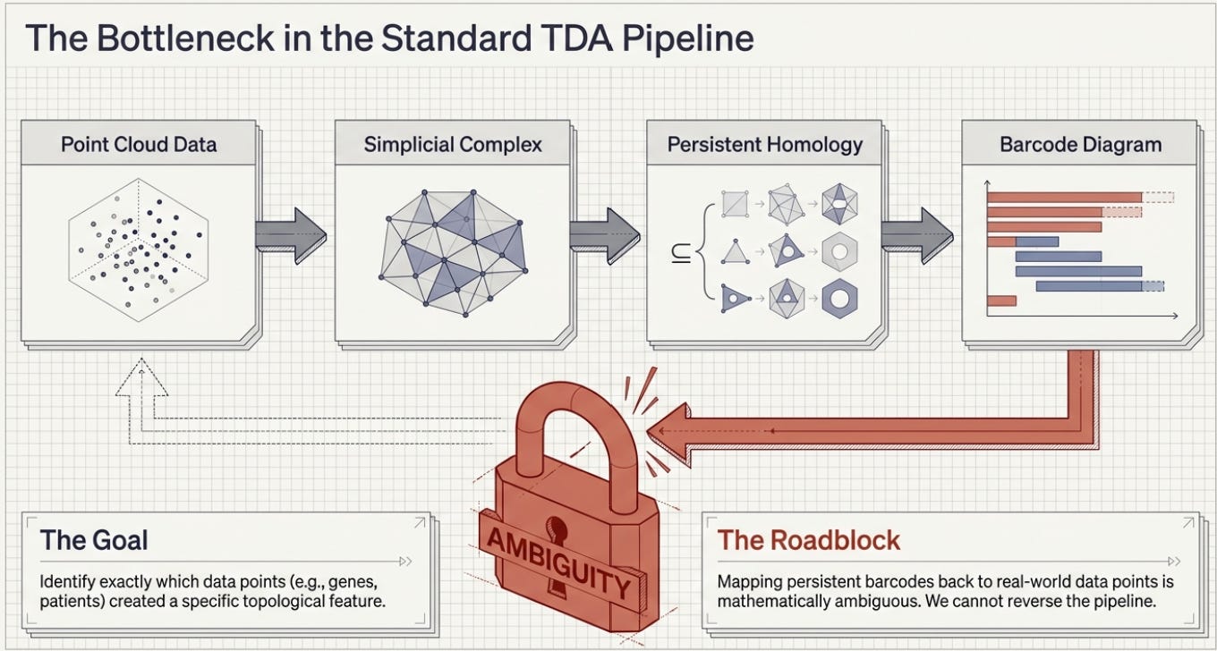
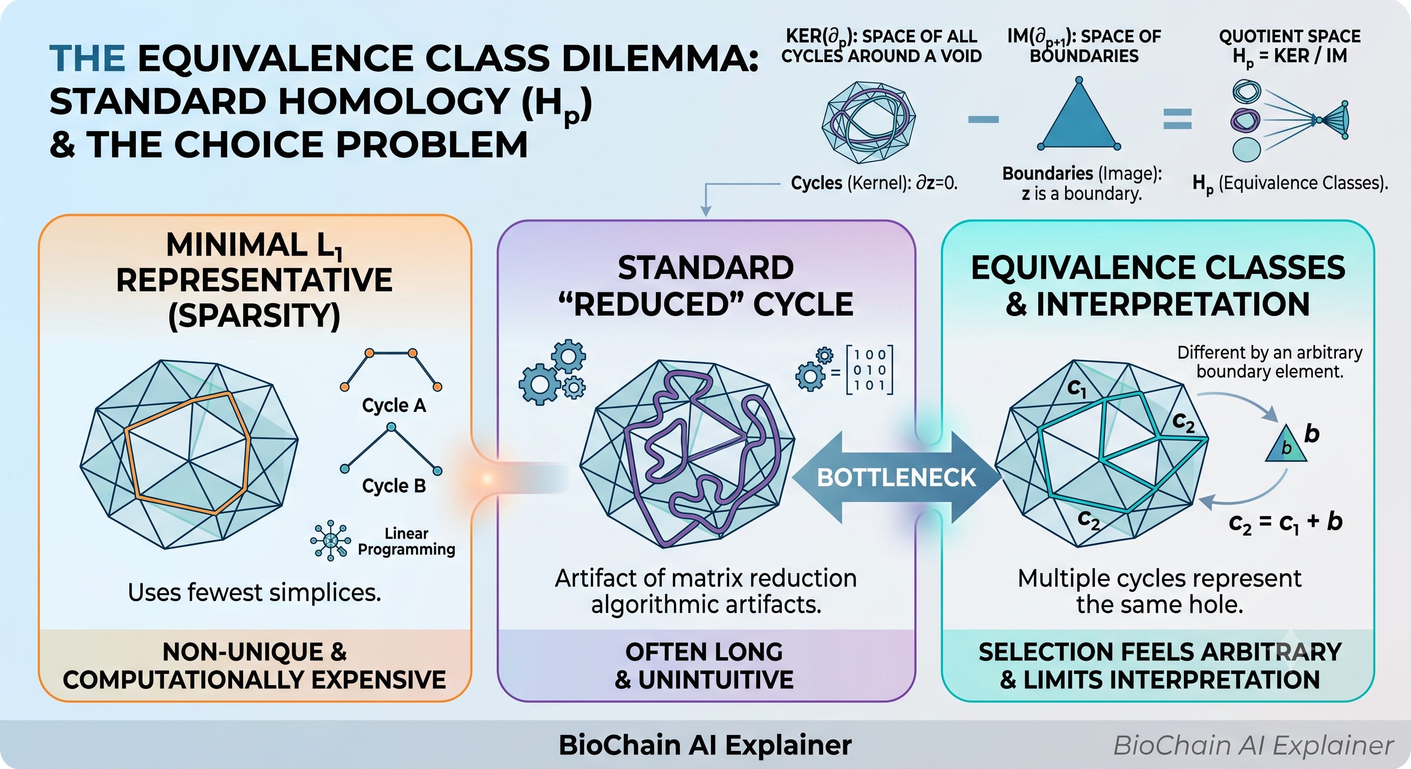
Traditional homology identifies these features as equivalence classes. This means that any two cycles are considered identical if they differ only by a “boundary” (a filled-in higher-dimensional shape). Consequently, there are mathematically infinite ways to draw a loop around a hole, making the choice of a “representative cycle” for biological interpretation feel arbitrary.
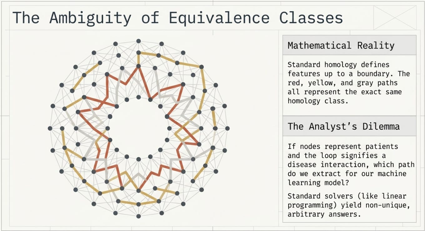
Concept Spotlight: The Uniqueness Problem In applied topology, we often seek the “best” representative for a homology class. While standard software provides a representative for free via matrix reduction, it is often a non-unique, “messy” cycle. Without a canonical choice, we cannot reliably map topological features back to specific data points for biomarker discovery.
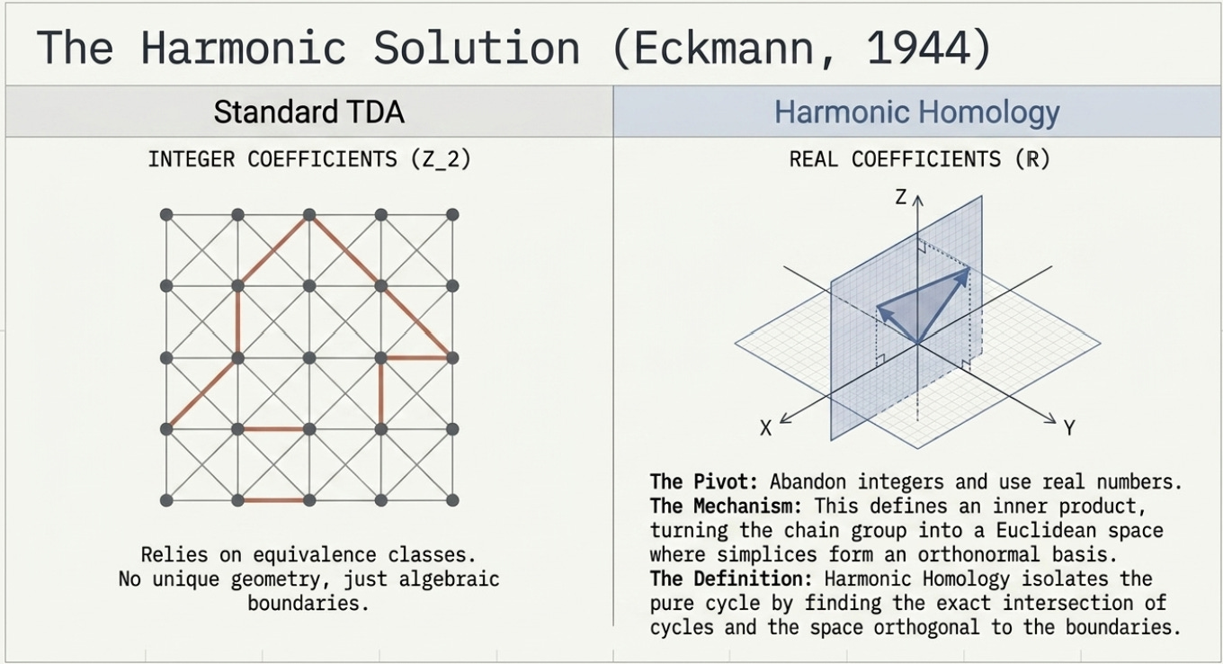
To solve this uniqueness problem and extract actionable insights, we must first build the geometric foundation upon which homology sits.
2. Building the Foundation: Simplicial Complexes and Filtration
The pipeline begins by transforming discrete data points into a continuous geometric shape called a simplicial complex. We denote the set of P-dimensional simplices (vertices, edges, triangles).
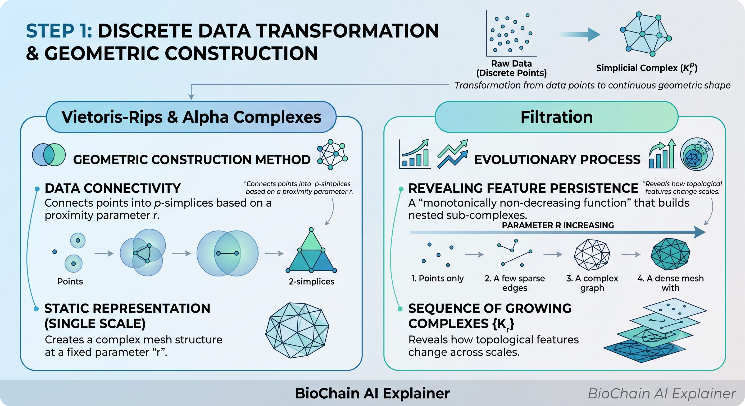
To compute homology, we must establish a rigorous orientation of the complex:
Vertex Ordering: We assume a strict ordering of the vertices (v_0, v_1,…, v_n).
Induced Simplex Ordering: This vertex ordering naturally induces an orientation for every p-simplex in the complex.
Chain Group Basis: These oriented simplices form the basis for our chain groups, allowing us to describe any cycle as a formal linear combination of simplices.
Once this structure is built, we need a mathematical language to describe the “holes” within it.
3. The Bottleneck: Equivalence Classes and the “Choice” Problem
We define the boundary map
to distinguish between different types of shapes:
Cycles (Kernel): Chains with no boundary
\((\partial z = 0)\)Boundaries (Image): Cycles that are the boundary of a (p+1)-simplex.
To pick a unique, canonical representative, we must move from abstract integers to the geometry of real-valued vector spaces.
4. The Harmonic Shift: Real Coefficients and Inner Products
In applied TDA, we typically use {Z}_2 coefficients. However, the harmonic approach utilizes real coefficients ({R}). While this may seem “weird” for discrete topology, it is technically necessary to turn the chain group into a Euclidean space.
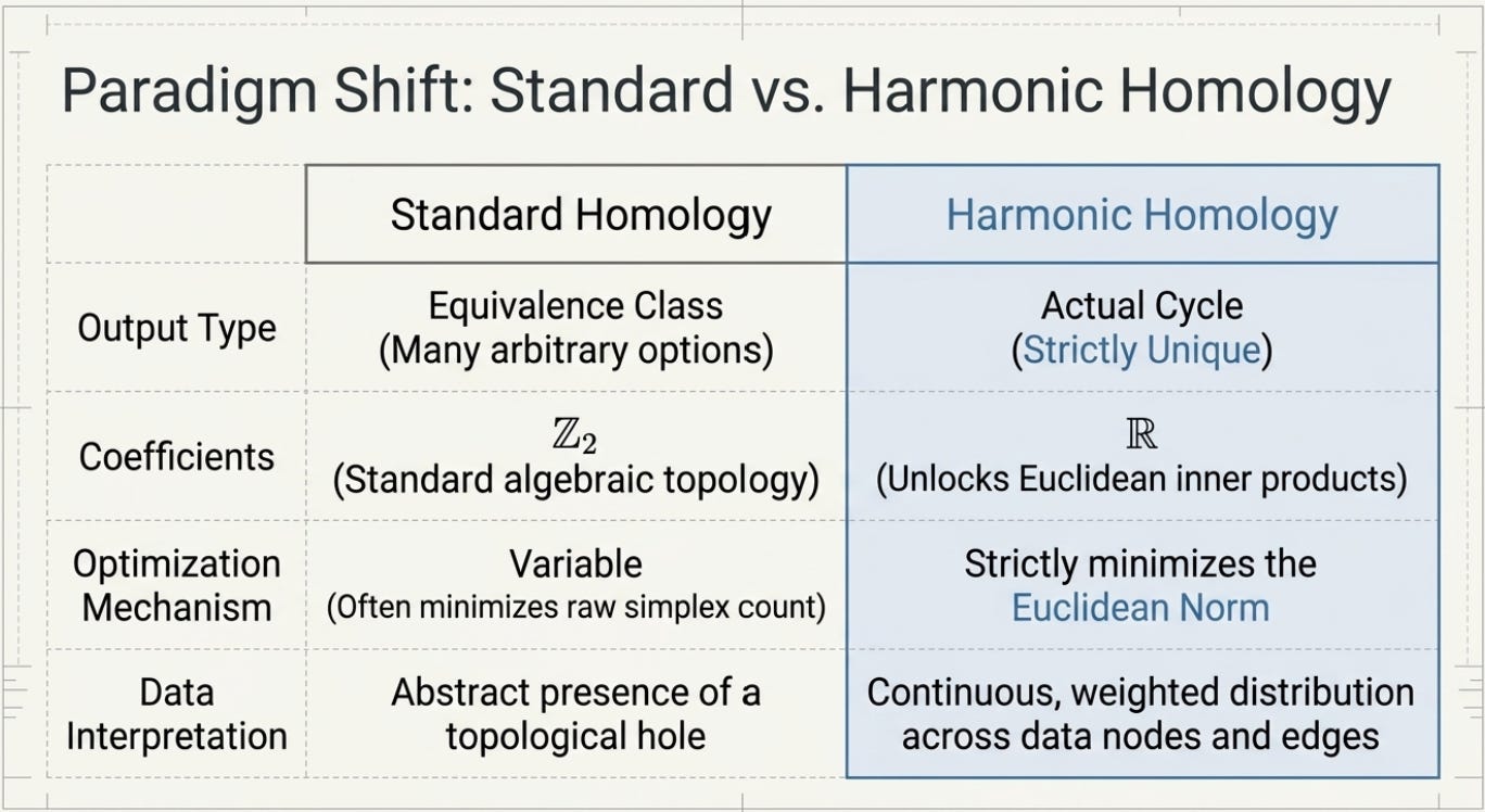
Defining the Inner Product: We declare the basis of all P-dimensional simplices to be an orthonormal basis. The scalar product
\(\langle \sigma_i, \sigma_j \rangle\)is 1 if i=j and 0 otherwise.
Establishing Orthogonality: This inner product allows us to define the “orthogonal complement” of a subspace.
The Harmonic Subspace: We define the Harmonic Homology Subspace
\((\mathcal\{Hp))\)as the intersection of the space of cycles and the space orthogonal to the boundaries:
\(\mathcal{H}p = \text{Ker}(~partial_p) \cap (\text{Im}(\partial_{p+1}))^\perp\)
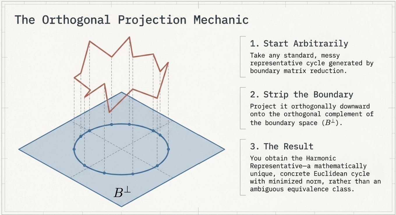
This shift allows us to project any messy representative cycle into a unique, optimal form residing in

5. Optimization: Essential Simplices and Norm Minimization
Within any homology class, some simplices are “essential.” An essential simplex is one that must be included in any cycle that loops around that specific hole; if removed, the cycle cannot close.
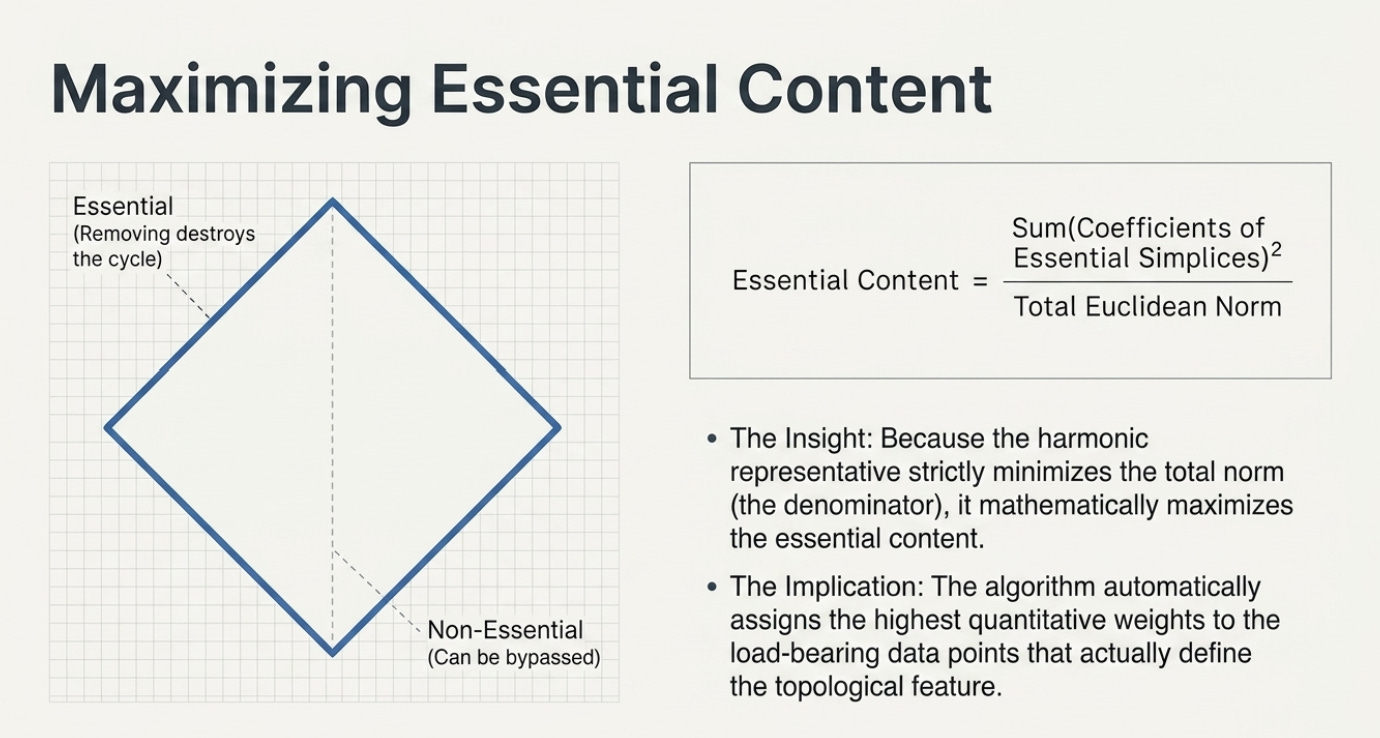
The Harmonic Representative is the unique cycle that minimizes the Euclidean (L_2) norm while maximizing the “relative essential content.”
Mathematical Insight: Relative Essential Content The harmonic representative z_h maximizes the following ratio:
Because zh minimizes the L_2 norm (the denominator) while maintaining the coefficients of essential simplices (which are already orthogonal to the boundary), it naturally highlights the most critical “non-negotiable” edges of the topological feature.
6. Diffusion and Calculation: The Harmonic Pipeline
Computationally, the harmonic representative acts as a Harmonic Flow. Much like current in a circuit, the weights “diffuse” across the complex. In this flow, the “circuit” around the hole is non-zero, but the “divergence” at each node is zero.
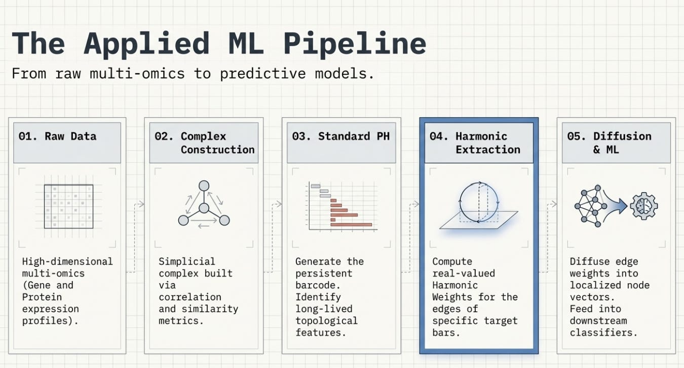
The Computational Pipeline Checklist:
[ ] Extract Representative: Obtain an initial cycle from standard boundary matrix reduction.
[ ] Compute Orthonormal Basis: Use the boundary matrix at the time of the bar’s birth to find a basis for the space of boundaries.
[ ] Project to Orthogonal Complement: Remove the “boundary component” of the cycle to find the L_2-minimal version.
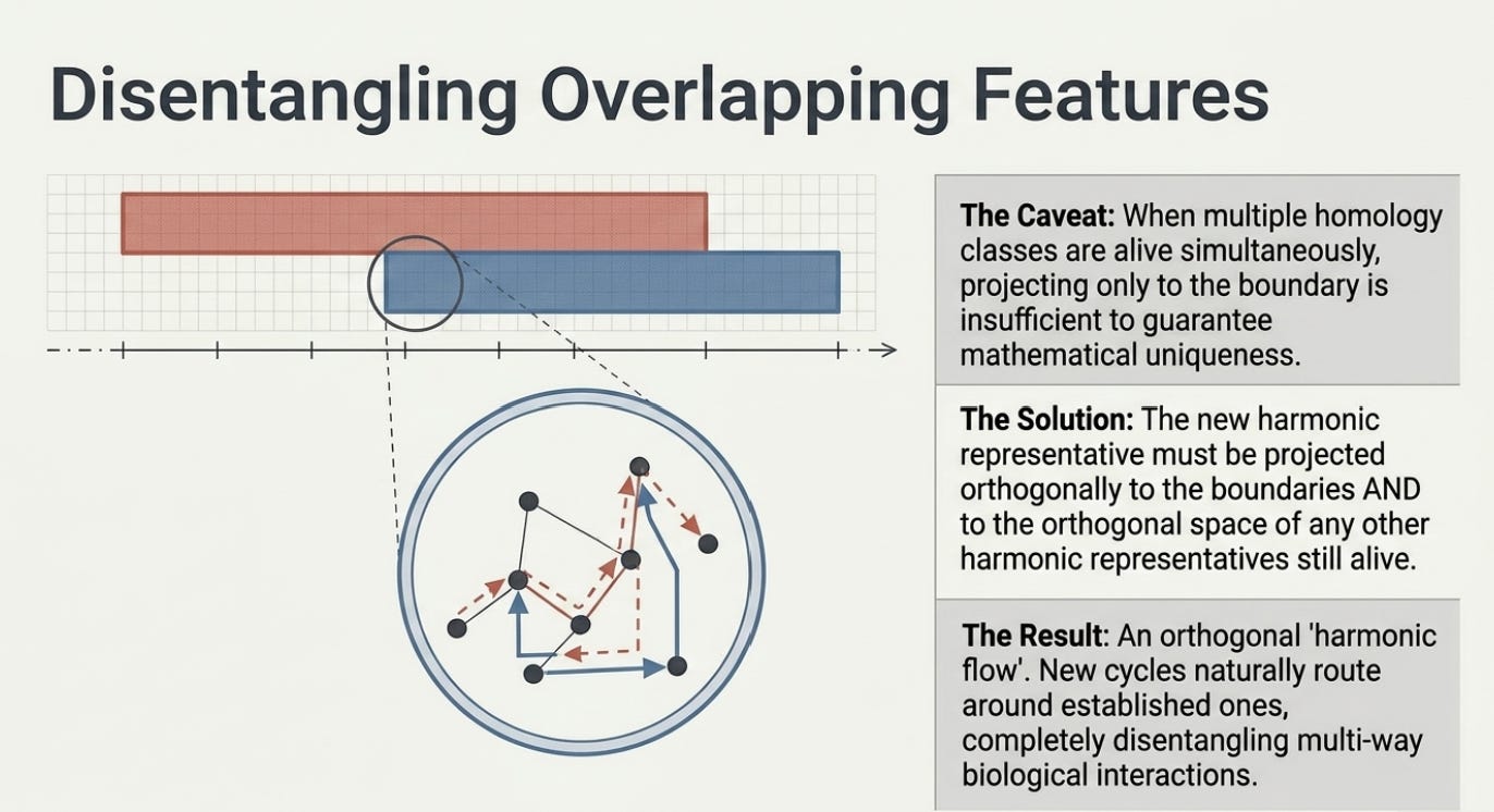
[ ] Disentangle Multi-way Interactions: If multiple bars (holes) overlap in the barcode, ensure the representative is orthogonal to all other “living” harmonic representatives to guarantee uniqueness.
This process results in harmonic weights assigned to edges and vertices, providing a canonical measurement of each data point’s contribution to a feature.
7. Real-World Impact: Biological Sample Patterning
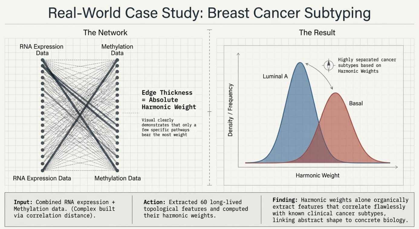
In computational biology, these weights transition from abstract topology to harmonic features. By aggregating weights from the edges onto the nodes (e.g., genes or patients), we create a new feature matrix for machine learning.
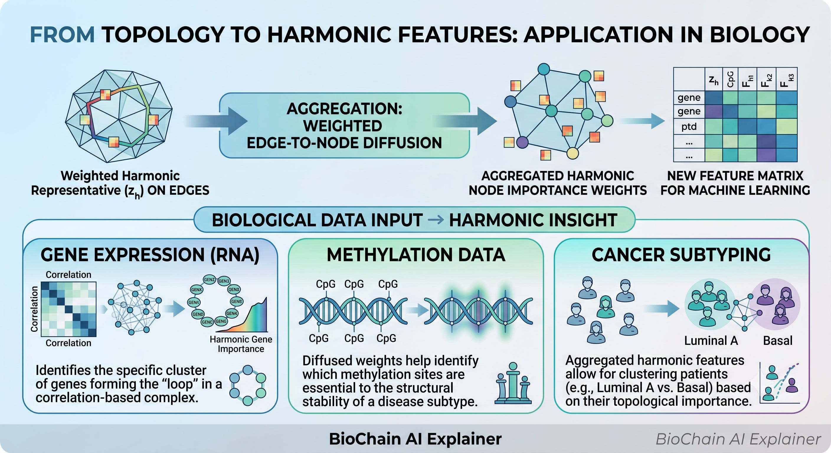
Aggregated harmonic features allow for clustering patients (e.g., Luminal A vs. Basal) based on their topological importance.
This “node diffusion” ensures that if an edge between two patients has a high harmonic weight, those patients are viewed as essential pillars of that topological signature.
8. Summary Checklist for the Learner
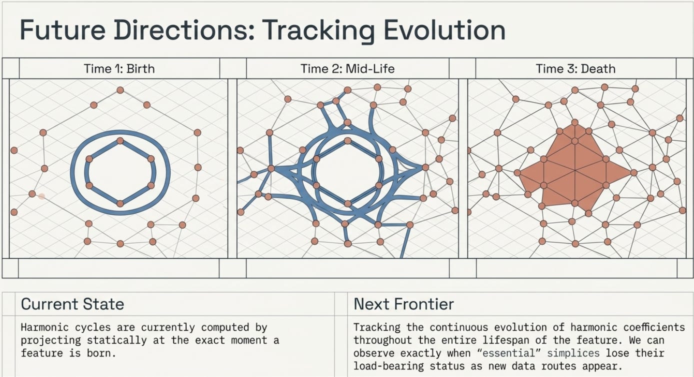
From Classes to Cycles: Harmonic TDA replaces ambiguous “equivalence classes” with a unique, canonical representative for every bar in a barcode.
Euclidean Optimization: By adopting real coefficients and L_2 norm minimization, we find the “minimal energy” representative that maximizes essential information.
Actionable Harmonic Features: The weights generated by the harmonic flow act as a bridge, allowing researchers to trace abstract “holes” back to the specific genes or samples that define them.
Check out my Patreon for implementation methods, and use-case Examples.